Introduction

The “Telecom Application Transaction Processing” benchmark was devised to model telco system behavior for benchmark purposes. The documentation describes it as follows:

The Telecommunication Application Transaction Processing (TATP) benchmark is designed to measure the performance of a relational DBMS/OS/Hardware combination in a typical telco application.

The benchmark generates a flooding load on a database server. This means that the load is generated up to the maximum throughput point that the server can sustain. The load is generated by issuing pre-defined transactions run against a specified target database. The target database schema is made to resemble a typical Home Location Register (HLR) database in a mobile phone network. The HLR is a database that mobile network operators use to store information about the subscribers and the services thereof.

While not well known, this benchmark is interesting for three reasons:

• It thinks in terms of business operations, instead of the ‘Gets’, ‘Puts’ and ‘Scans’ you see in NoSQL focused examples.
• It’s a good example of the “Alternative Unique Key” problem.
• It’s reasonable model of a Home Location Registry, which is an important real world system that almost everyone uses every day.

The “Alternative Unique Key” problem

Over the last decade we’ve seen a shift away from every bigger servers to private clouds filled with commodity hardware. As part of this shift database providers have responded by making new products that are horizontally sharded – instead of all servers trying to ‘know’ about all the data an algorithm is used to send it to 2 or more of them, who effectively ‘own’ it. So while a cluster might have 30 nodes, only 2 or 3 of them might actually have access to a given record, depending on how many copies you’d decided to keep.

Obviously this approach depends on being able to figure out where a record belongs, which in turn implies that you know the Primary Key of your record. “Key value” stores are a great example of this approach in action – finding a record if you know the key is really fast.

In cases where you are using a conventional Foreign Key value – such as ‘Zipcode’ or ‘State’ – you can still get data by asking all 30 nodes, as these low cardinality foreign keys imply many possible matches and asking all 30 nodes is thus a reasonable thing to do. In real life ‘zipcode’ or ‘state’ queries that return 1000’s of rows aren’t that common in OLTP systems, and when they are you can usually mitigate the issue by prepending them to the Primary Key, which limits where your rows can end up. Volt Active Data also has “Materialized Views” which can efficiently keep running totals for “Count(*)” queries of this nature.

But what happens if have to work with an identifier which is an alternative Unique Key?, Like the primary key it uniquely identifies a record, but it comes from a different ‘namespace’ to the one you use 80% of the time, and can change every couple of minutes? You don’t know where to look, and asking all 30 nodes in your cluster isn’t very efficient. It turns out this scenario is very common in the telecoms industry, where pretty much everything you speak to will give you an identifier it owns and manages at the start of every interaction, and will insist on using it for the rest of the interaction. This means you’ll get lots of messages referring to an id that is unique at that moment in time, but is of no use to you when it comes to finding the underlying record you are talking about.

What makes the TATP benchmark interesting is that fully 20% of the transactions are like this.

There is no “Correct” answer to the “Alternative Unique Key” Problem

From an implementation perspective this is a non-trivial problem. It’s not a Volt Active Data-specific problem. All horizontally sharded systems will have to make some awkward choices. The default list generally looks like this:

1. Use a single, large server running a legacy RDBMS so you can do the search and write in one move.

This simply isn’t going to work if you are obliged by the market to deploy on smaller, commodity hardware. In addition, most NoSQL/NewSQL products are around 10x faster than a legacy RDBMS. So a workload that would require 3 generic servers for NoSQL/NewSQL won’t need single server with 3x the power for a legacy RDBMS, it’ll need to be 30x the power. Unsurprisingly, we don’t bother testing this in our implementation.

2. Maintain a separate index table/KV store and write to both at the same time.

In the example below the Primary Key lives on Node 1. We create an index entry which looks like another record to the database. For our purposes the index record lives on Node 2.

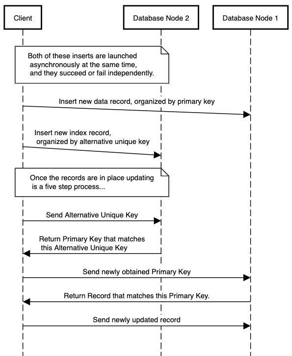
This will work and scale well, but has two serious problems:

• Both reads and writes are now a two step process. There are a whole series of edge case scenarios where (for example) reads can’t find a row that exists because they looked at the secondary index 500 microseconds too early. Depending on your application this may not matter. For the “Telecom Application Transaction Processing” Use Case we could probably get away with it, as the FK involves roaming users and it’s hard for phone users to change their roaming status multiple times per second.
• The real problem is the complexity around error handling. What happens if one write works, but another fails? How do I “uncorrupt” the data? What do I do with incoming requests in the meantime? For these reasons we don’t bother testing this in our implementation, although we might add this in a future iteration.

3. Get your NewSQL/NoSQL store to do a global search, then do a write.

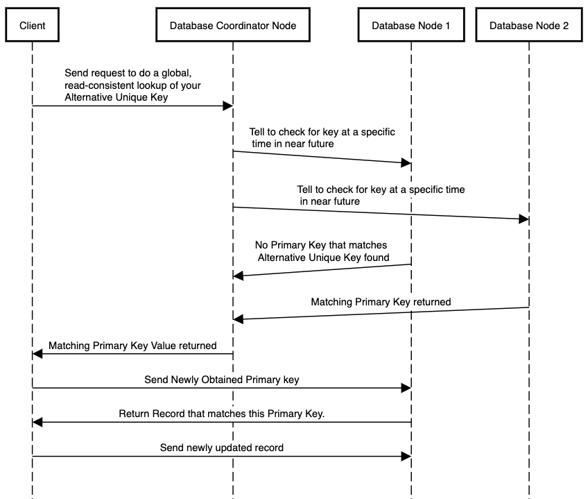
This assumes that there is such a thing as a global read in your environment. In Volt Active Data we handle this behind the scenes, but a single node will still be in charge of getting the other nodes to issue the query at the exact same moment in time. The “FKMODE_MULTI_QUERY_FIRST” option in our implementation does such a read to turn the foreign key into a subscriber id, which is then used for the actual transaction. Under normal circumstances both events take well under a millisecond to complete, which means the time window when things can go wrong is very small.  The downside from a Volt Active Data perspective is that while what we call “Multi Partition Reads” are fast, they aren’t nearly as fast as single partition transactions. 

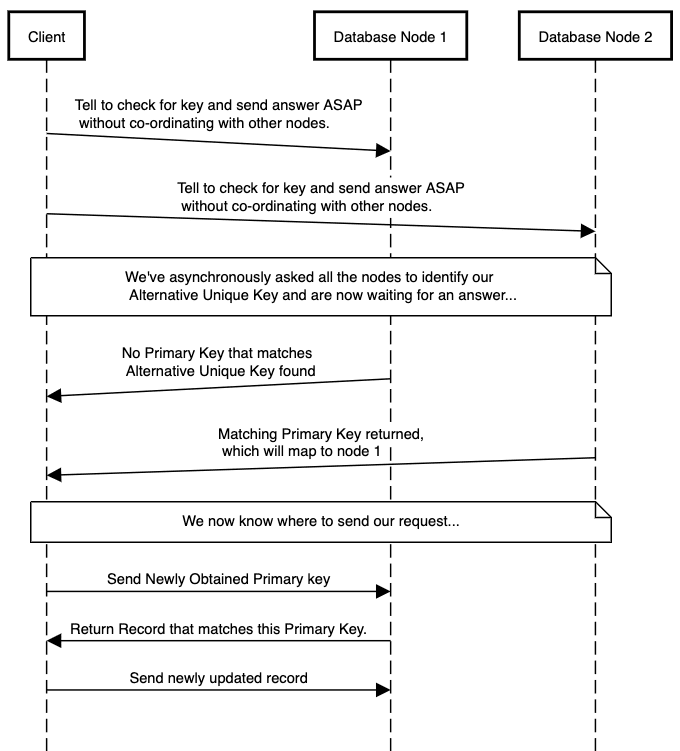
4. Do a ‘read’ to ask all possible locations if they recognize your unique key, one at a time.

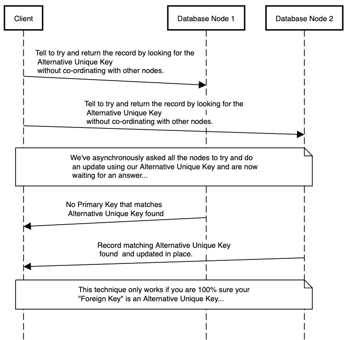
This is a variation on step ‘4’, except we just send ‘writes’ to attempt to do the update in every possible location. In our implementation this is the “FKMODE_TASK_ALL_PARTITIONS” option. On the face of it this seems to be a classic case of ‘write amplification’, but from a Volt perspective ‘reads’ and ‘writes’ both cost roughly the same to do. It also has the advantage that being one step we can’t be flummoxed by the unique key being updated, provided it isn’t instantly assigned to someone else. We know from the Use Case this won’t happen.

We go into detail about how our implementation works below, but a key takeaway is that not only is this a hard problem to solve, but the different possible solutions are all ‘optimal’ depending on your use case.

You can do your transaction once you know the subscriber_id, so as a prerequisite you get the subscriber id by asking everyone if they recognize your Unique Key. This seems slightly crazy, but is actually viable, provided you’re not trying to do this for every transaction. Obviously it creates problems for scalability, but before panicking we should see what kind of numbers we get and see if this is actually an issue. In the TATP benchmark 20% of transactions fall into this category. In our implementation this is the “FKMODE_QUERY_ALL_PARTITIONS_FIRST” option.

5. Ask all possible locations to do the update if they have an entry that matches the Unique Key.

The TATP Schema

The Schema looks like this:

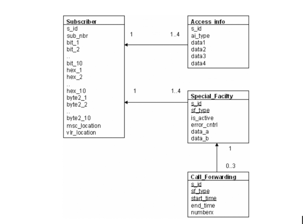
The documentation defines it as the following tables:

Subscriber Table

1. s_id is a unique number between 1 and N where N is the number of subscribers (the population size).Typically, the population sizes start at N=100,000 subscribers, and then N is multiplied by factors of 2, 5 and 10 and so forth, for each order of magnitude. During the population, s_id is selected randomly from the set of allowed values.
2. sub_nbr is a 15 digit string. It is generated from s_id by transforming s_id to string and padding it with leading zeros. For example: s_id 123 sub_nbr “000000000000123”
3. bit_X fields are randomly generated values (either 0 or 1).
4. hex_X fields are randomly generated numbers between 0 and 15.
5. byte2_X fields are randomly generated numbers between 0 and 255.
6. sc_location and vlr_location are randomly generated numbers between 1 and (232 – 1).

Access_Info Table

1. s_id references s_id in the Subscriber table.
2. ai_type is a number between 1 and 4. It is randomly chosen, but there can only be one record of each ai_type per each subscriber. In other words, if there are four Access_Info records for a certain subscriber they have values 1, 2, 3 and 4.
3. data1 and data2 are randomly generated numbers between 0 and 255.
4. data3 is a 3-character string that is filled with random characters created with upper case A-Z letters.
5. data4 is a 5-character string that is filled with random characters created with upper case A-Z letters.

There are between 1 and 4 Access_Info records per Subscriber record, so that there are 25 % subscribers with one record, 25% with two records and so on.

Special_Facility Table

1. s_id references s_id in the Subscriber table.
2. sf_type is a number between 1 and 4. It is randomly chosen, but there can only be one record of each sf_type per each subscriber. So if there are four Special_Facility records for a certain subscriber, they have values 1, 2, 3 and 4.
3. is_active is either 0 or 1. is_active is chosen to be 1 in 85% of the cases and 0 in 15% of the cases.
4. error_cntrl and data_a are randomly generated numbers between 0 and 255.
5. data_b is a 5-character string that is filled with random characters created with upper case A-Z letters.

There are between 1 and 4 Special_Facility records per row in the Subscriber table, so that there are 25% subscribers with one record, 25% with two records and so on.

Call_Forwarding Table

1. s_id and sf_type reference the corresponding fields in the Special_Facility table.
2. start_time is of type integer. It can have value 0, 8 or 16 representing midnight, 8 o’clock or 16 o’clock.
3. end_time is of type integer. Its value is start_time + N, where N is a randomly generated value between 1 and 8.
4. numberx is a randomly generated 15 digit string.

There are between zero and 3 Call_Forwarding records per Special_Facility row, so that there are 25 % Special_Facility records without a Call_Forwarding record, 25% with one record and so on. Because start_time is part of the primary key, every record must have different start_time.

Initial Data

The database is always freshly populated before each benchmark run. This ensures that runs are reproducible, and that each run starts with correct data distributions. The Subscriber table acts as the main table of the benchmark. After generating a subscriber row, its child records in the other tables are generated and inserted. The number of rows in the Subscriber table is used to scale the population size of the other tables. For example, a TATP with population size of 1,000,000 gives the following table cardinalities for the benchmark:

• Subscriber = 1,000,000 rows
• Access_Info ≈ 2,500,000 rows
• Special_Facility ≈ 2,500,000 rows
• Call_Forwarding ≈ 3,750,000 rows

Transaction mixes

The basic TATP benchmark runs a mixture of seven (7) transactions issued by ten (10) independent clients. All the clients run the same transaction mixture with the same transaction probabilities as defined below.

Read Transactions (80%)

• GET_SUBSCRIBER_DATA 35 %
• GET_NEW_DESTINATION 10 %
• GET_ACCESS_DATA 35 %

Write Transactions (20%)

• UPDATE_SUBSCRIBER_DATA 2 %
• UPDATE_LOCATION 14 %
• INSERT_CALL_FORWARDING 2 %
• DELETE_CALL_FORWARDING 2 %

Volt Active Data Implementation

From a Volt Active Data viewpoint the challenge here is how to handle transactions that access via sub_nbr instead of the partitioned key s_id.
The following transactions access via the partitioned key and are trivial to implement in Volt Active Data:

• GetSubscriberData
• GetNewDestination
• GetAccessData
• UpdateSubscriberData

These transactions represent 20% of the logical transactions, but use the synthetic Unique Key mandated by the benchmark:

• UpdateLocation
• InsertCallForwarding
• DeleteCallForwarding

From a Volt Active Data viewpoint our design choices were discussed above. We implemented the following:

• “FKMODE_MULTI_QUERY_FIRST” does a global read consistent query to find the row, and then follows up with a single partition update.
• “FKMODE_QUERY_ALL_PARTITIONS_FIRST” asks each partition independently to find the row, and then follows up with a single partition update.
• “FKMODE_TASK_ALL_PARTITIONS” cuts out the middleman and asks each partition independently to try and update the row. Given that there is only one row and while the Unique ID is volatile it doesn’t get reused this will work for this specific Use Case.
• What our benchmark does

Our code stats by creating the test data if needed. It then runs our version of the benchmark for each implementation for 5 minutes. It starts at 2,000 TPS and then re-runs with 4,000, 6,000 , etc until the server can no longer get > 90% of requested transactions done or we hit some other reasons for stopping. We then look at the previous file and use the TPS it did as the result for that configuration. It does this for each of the three methods we discuss above. We produce an output log file which has detailed statistics for 1 of the 10 threads.

Volt Active Data results in AWS

Configuration

For testing purposes we ran all 3 options above on the following configuration:

• AWS
• z1d.2xlarge – Intel Xeon, runs up to ‘up to 4.0 GHz’, 4 physical cores per server. Around US$0.25/hr.
• 3 nodes
• k=1 (1 spare copy)
• Snapshotting and command logging enabled.

Note that:

• All our transactions are ACID transactions
• ‘k=1’ ensures that all transactions take place on 2 nodes.
• ‘z1d.2xlarge’ has 8 vCPUs, or 4 real ones.

Results

The best result was obtained was when we asked all the partitions to do a read and then do an update once we’ve found out where it is (FKMODE_QUERY_ALL_PARTITIONS_FIRST). We were able to sustain 66,635 TPS while aiming for 68K. At that level the hardware wasn’t maxed out, but the 99th percentile latency for our tricky “Alternative Unique Key” was still around 1ms. As we increased the workload it jumped to over 10ms, which is the point at which it will not be acceptable to customers.

The next best alternative for the “Alternative Unique Key” stuff is to ask all the partitions to try and do it. We were able to get 27,518 TPS by the time latency reached 10ms. This does, however, have the advantage of not having to worry about updates.

The worst outcome was for using a multi partition query. The additional overhead comes from making sure that all nodes issue the query at the exact same moment in time.

Note that at 66,635 TPS for basic read and write operations latency is still 1ms or under at this point.

In the graph below the X axis is the load we requested, the thick blue line is how ahy TPS we’re doing (right axis). The performance of individual operations is on the left hand scale in milliseconds. Note that if for some reason you didn’t care about latency you could get something more than 100K TPS.

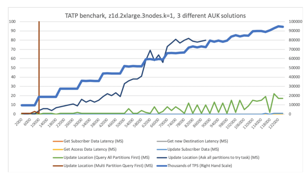
Bear in mind this is on a generic AWS configuration without making any heroic attempts to maximize performance. Our goal is to create something that people evaluating Volt Active Data can do for themselves.This is not – and does not claim to be – the ‘most’ Volt Active Data can get on this benchmark or on AWS.

How to run this yourself

1. Download and install Volt Active Data
2. All the code is in github (https://github.com/srmadscience/voltdb-tatpbenchmark) and is a maven project. So getting it is a case of:
   git clone https://github.com/srmadscience/voltdb-tatpbenchmark
   cd voltdb-tatpbenchmark
3. The script runbenchmark does a build, and then installs the schema and starts the benchmark:

sh scripts/runbenchmark.sh

‘Runbenchmark.sh’ can be run with three parameters:

• Hosts – comma delimited list of volt servers. Defaults to the hostname.
• Testname – a word describing the purpose of the test. Defaults to the hostname.
• Subscribers – How many subscribers should be in your Home Location Registry. 1,000,000 subs takes about 600MB of RAM. We ran our tests with 20,000,000.

So an example would be:

sh scripts/runbenchmark.sh vdb1,vdb2,vdb3 mytest 20000000